Phylogenetic analysis of the threshold model

1. We're going to estimate the correlation between two binary characters, as well as between a binary & a continuous character, assuming a threshold model of character evolution for our discrete character; and
2. We're going to reconstruct the ancestral states of a multistate, naturally ordered character on the tree assuming the threshold model.

If you want to follow along without actually running the simulation and the MCMC, you can download the following R data object: threshold.Rdata.

Correlation between discrete & continuous characters under the threshold model

Here, we're going to use Bayesian MCMC to sample the evolutionary parameters of our model from their joint posterior probability distribution. These parameters include evolutionary rates (σ²s) for each continuous character; and the correlation between our discrete and continuous character. Since this is a binary model with a single threshold - we don't have to worry about the relative positions of the thresholds.

We'll start by simulating a tree & two correlated Brownian variables on the tree.

For illustrative purposes, let's start by using threshBayes on two continuous characters & show that the result lines up closely with our MLE of the correlation.

## first, load phytools
library(phytools)
tree <- pbtree(n = 100, scale = 1)
r <- 0.75  # simulate using a high correlation
V <- matrix(c(1, r, r, 1), 2, 2)
X <- sim.corrs(tree, V)
## set some parameters for the MCMC
sample <- 1000
ngen <- 5e+05
burnin <- 0.2 * ngen
## we can start by running our Bayesian MCMC on the original data
AA <- threshBayes(tree, X, types = c("cont", "cont"), ngen = ngen, control = list(sample = sample))

## [1] "gen 1000"
## [1] "gen 2000"
## [1] ...
## [1] "gen 500000"

## we can compute our MLE of the correlation
V.mle <- phyl.vcv(X, vcv(tree), lambda = 1)$R
V.mle[1, 2]/sqrt(V.mle[1, 1] * V.mle[2, 2])

## [1] 0.761

## here is our 'post burnin' mean from the posterior sample
mean(AA$par[(burnin/sample + 1):nrow(AA$par), "r"])

## [1] 0.755

## plot our likelihood profile
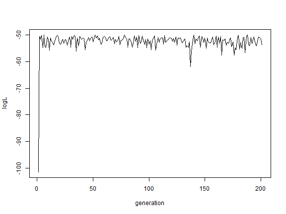
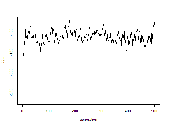
plot(AA$par[, "logL"], type = "l", xlab = "generation", ylab = "logL")

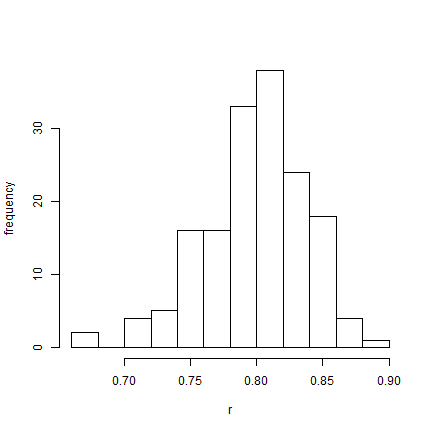
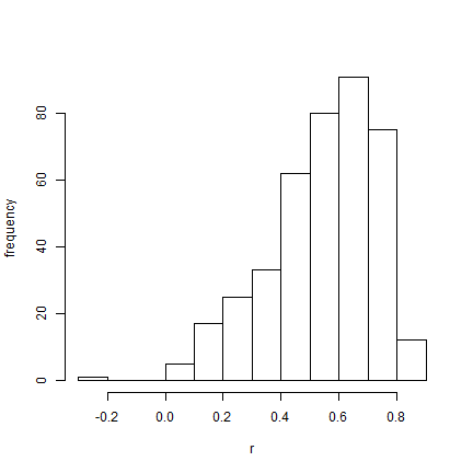
## plot our posterior sample for the correlation
hist(AA$par[(burnin/sample + 1):nrow(AA$par), "r"], xlab = "r", ylab = "frequency", 
    main = NULL)

OK, this was just a proof-of-concept exercise. Now let's try the same thing after having converted one of our trait values into a threshold character.

## convert X[,2] to a binary character
X[, 2] <- as.numeric(sapply(X[, 2], threshState, thresholds = setNames(c(0, 
    Inf), 0:1)))
BB <- threshBayes(tree, X, types = c("cont", "disc"), ngen = ngen, control = list(sample = sample))

## [1] "gen 1000"
## [1] "gen 2000"
## [1] ...
## [1] "gen 500000"

## what is our estimate of the correlation?
mean(BB$par[(burnin/sample + 1):nrow(BB$par), "r"])

## [1] 0.5804

## plot our likelihood profile
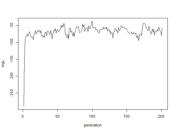
plot(BB$par[, "logL"], type = "l", xlab = "generation", ylab = "logL")

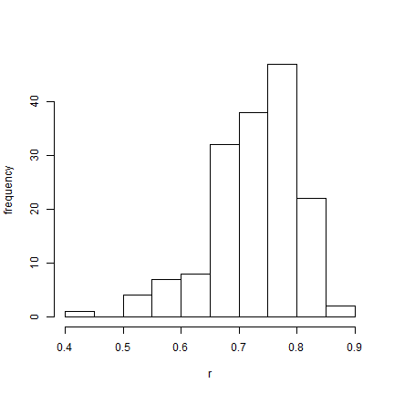
## plot our posterior sample for the correlation
hist(BB$par[(burnin/sample + 1):nrow(BB$par), "r"], xlab = "r", ylab = "frequency", 
    main = NULL)

Finally, let's analyze two binary characters under the same model. Remember, each time we're losing information about the underlying correlation between liabilities. Nonetheless....

## convert X[,2] to a binary character
X[, 1] <- as.numeric(sapply(X[, 1], threshState, thresholds = setNames(c(0, 
    Inf), 0:1)))
CC <- threshBayes(tree, X, types = c("disc", "disc"), ngen = ngen, control = list(sample = sample))

## [1] "gen 1000"
## [1] "gen 2000"
## [1] ...
## [1] "gen 500000"

## what is our estimate of the correlation?
mean(CC$par[(burnin/sample + 1):nrow(CC$par), "r"])

## [1] 0.5456

## plot our likelihood profile
plot(CC$par[, "logL"], type = "l", xlab = "generation", ylab = "logL")

## plot our posterior sample for the correlation
hist(CC$par[(burnin/sample + 1):nrow(CC$par), "r"], xlab = "r", ylab = "frequency", 
    main = NULL)

So we can see that we can see that threshBayes does a reasonable job at estimating the correlation between binary & continuous characters under the threshold model.

## let's use coda to compute effective sample sizes & HPDs
require(coda)

## Loading required package: coda

## first, analysis A
rA <- AA$par[(burnin/sample + 1):nrow(AA$par), "r"]
class(rA) <- "mcmc"
effectiveSize(rA)

## var1 
##  401

HPDinterval(rA)

##      lower  upper
## var1 0.663 0.8319
## attr(,"Probability")
## [1] 0.9501

## second, analysis B
rB <- BB$par[(burnin/sample + 1):nrow(BB$par), "r"]
class(rB) <- "mcmc"
effectiveSize(rB)

##  var1 
## 35.78

HPDinterval(rB)

##       lower  upper
## var1 0.3522 0.8179
## attr(,"Probability")
## [1] 0.9501

## finally, analysis C
rC <- CC$par[(burnin/sample + 1):nrow(CC$par), "r"]
class(rC) <- "mcmc"
effectiveSize(rC)

##  var1 
## 37.51

HPDinterval(rC)

##       lower  upper
## var1 0.1622 0.8076
## attr(,"Probability")
## [1] 0.9501

Ancestral character estimation under the threshold model

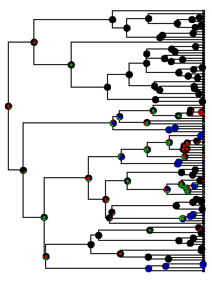
We can also do ancestral character reconstruction for discrete characters using the threshold model.

## simulate tree & data
n <- 100
ngen <- 1e+06
sample <- 1000
tree <- pbtree(n = n, scale = 10)
x <- fastBM(tree, sig2 = 1, a = 0.5, internal = TRUE)
th <- sapply(x, threshState, thresholds = setNames(c(0, 0.5, 2, Inf), letters[1:4]))
mcmc <- ancThresh(tree, th[1:n], ngen = ngen, sequence = letters[1:4], control = list(sample = sample, 
    plot = FALSE))

## MCMC starting....

## gen 1000

...

## gen 999000

## gen 1000000

plotTree(tree, setEnv = TRUE, ftype = "off")

## setEnv=TRUE is experimental. please be patient with bugs

tiplabels(pie = to.matrix(th[1:n], letters[1:4]), piecol = palette()[1:4], cex = 0.3)
nodelabels(pie = mcmc$ace, piecol = palette()[1:4], cex = 0.8)
nodelabels(pie = to.matrix(th[1:tree$Nnode + n], letters[1:4]), piecol = palette()[1:4], 
    cex = 0.4)

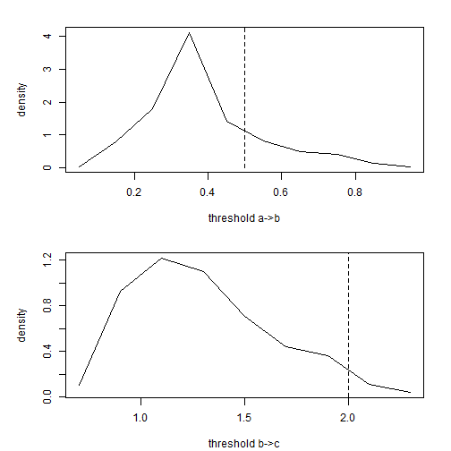
Theoretically, we can even use this method to identify the relative positions of thresholds:

colMeans(mcmc$par[(0.2 * ngen/sample):(ngen/sample) + 1, letters[1:4]])

##      a      b      c      d 
## 0.0000 0.3878 1.2953    Inf

par(mfrow = c(2, 1))
par(mar = c(4.1, 5.1, 2.1, 2.1))
xx <- hist(mcmc$par[(0.2 * ngen/sample):(ngen/sample) + 1, letters[2]], plot = FALSE)
plot(xx$mids, xx$density, type = "l", xlab = "threshold a->b", ylab = "density")
lines(c(0.5, 0.5), c(0, 1.1 * max(xx$density)), lty = "dashed")
xx <- hist(mcmc$par[(0.2 * ngen/sample):(ngen/sample) + 1, letters[3]], plot = FALSE)
plot(xx$mids, xx$density, type = "l", xlab = "threshold b->c", ylab = "density")
lines(c(2, 2), c(0, 1.1 * max(xx$density)), lty = "dashed")