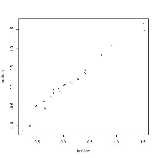
aa <- fastAnc(tree, x) plot(aa, RR$par[2:length(RR$par)], xlab = "fastAnc", ylab = "custom")
For better or for worse, the estimation of phenotypic trait values for ancestral nodes in the tree continues to be an important goal in phylogenetic comparative biology.
In this tutorial, I focus on the following five topics:
1. Estimating the ancestral states of continuous characters.
2. Visualizing continuous character ancestral states for one or multiple
traits.
3. Estimating ancestral character states for discrete characters under a
continuous-time Markov chain.
4. Simulating stochastic character histories for a discrete character
(stochastic character mapping).
5. Simultaneously plotting discrete & continuous character
reconstructions.
To estimate the states for a continuously valued character at ancestral nodes in the tree, we need to maximize the states at the internal nodes of tree which we expect to have a multivariate normal distribution.
This is relatively simple in principle. For instance, in the code below - I
have taken advantage of the functions of "phytools" and another
R package called "mnormt" to compute the joint likelihood of our
Brownian rate (σ2)** and our states at all the internal nodes of
the tree.
(**Note that the fitted Brownian rate is not the same as the MLE of σ2 conditioning only on the states for the tips of the tree. The rate estimated here will be too low because it treats the states at internal nodes as known, and then conditions on these states.)
## set seed for reproducibility
set.seed(100)
## load phytools
library(phytools)
## simulate a tree & some data
tree <- pbtree(n = 26, scale = 1)
tree$tip.label <- LETTERS[26:1]
x <- fastBM(tree)
## let's try & write down the likelihood function we want
C <- vcvPhylo(tree)
pp <- rep(1, tree$Nnode + 1)
lik <- function(pp, C, x) -sum(dmnorm(c(x, pp[3:length(pp)]), rep(pp[2], nrow(C)),
    pp[1] * C, log = TRUE))
tt <- setNames(c(1, rep(mean(x), tree$Nnode)), c("sig2", 1:tree$Nnode + length(tree$tip)))
RR <- optim(tt, lik, C = C, x = x, method = "L-BFGS-B", lower = c(1e-06, rep(-Inf,
    tree$Nnode)))
print(RR)
## $par
##      sig2        27        28        29        30        31        32
##  0.000001  0.360920  1.677493  1.472784  0.117096  0.051251  0.043723
##        33        34        35        36        37        38        39
##  0.067812 -0.063631 -1.014297 -1.141446 -0.159674 -0.271753 -0.559683
##        40        41        42        43        44        45        46
## -0.115334 -0.189465  0.202020  0.214177  0.435215  0.833868  1.109123
##        47        48        49        50        51
## -0.056934 -0.374485 -0.498910 -0.372938  0.116875
##
## $value
## [1] 18893643
##
## $counts
## function gradient
##       13       13
##
## $convergence
## [1] 0
##
## $message
## [1] "CONVERGENCE: REL_REDUCTION_OF_F <= FACTR*EPSMCH"
The problem with this method is that it will generally be inefficient at finding the ML solution as the number of nodes in our tree increases, and will even often fail to find the MLE. Luckily some R packages have more efficient methods for finding the same MLEs of ancestral nodes. Here is an example, and we can use it to "truth" our optimization, shown above:
aa <- fastAnc(tree, x)
plot(aa, RR$par[2:length(RR$par)], xlab = "fastAnc", ylab = "custom")

We can also use fastAnc to get 95% CIs on ancestral state values,
given our model - as follows:
AA <- fastAnc(tree, x, CI = TRUE)
print(AA)
## $ace
##         27         28         29         30         31         32
##  0.4038429  1.5060325  1.5131013  0.1696467  0.0092989 -0.0009378
##         33         34         35         36         37         38
##  0.0265075 -0.2029285 -0.6334198 -0.7574224 -0.1916646 -0.2394627
##         39         40         41         42         43         44
## -0.3508794 -0.0562375 -0.1880745  0.2740616  0.2787586  0.4038396
##         45         46         47         48         49         50
##  0.7171769  0.9055803 -0.0958945 -0.3002784 -0.5135732 -0.3683351
##         51
##  0.1456773
##
## $CI95
##       [,1]     [,2]
## 27 -0.6686  1.47629
## 28  1.2191  1.79292
## 29  1.2925  1.73371
## 30 -0.6300  0.96929
## 31 -0.5995  0.61814
## 32 -0.5759  0.57399
## 33 -0.5412  0.59421
## 34 -0.8298  0.42399
## 35 -1.1754 -0.09142
## 36 -1.2020 -0.31288
## 37 -0.7036  0.32023
## 38 -0.7401  0.26118
## 39 -0.7633  0.06153
## 40 -0.5202  0.40770
## 41 -0.5368  0.16066
## 42 -0.3209  0.86905
## 43 -0.3389  0.89645
## 44 -0.2178  1.02550
## 45  0.1164  1.31797
## 46  0.3304  1.48079
## 47 -0.7395  0.54768
## 48 -1.0083  0.40776
## 49 -0.6071 -0.42006
## 50 -0.4589 -0.27776
## 51 -0.7051  0.99646
These CIs could theoretically be used to test hypotheses about ancestral state estimates for internal nodes.
There are some convenient ways to visualize ancestral state reconstructions on the phylogeny.
The simplest type of ancestral character visualization is a method called the traitgram. In this method, we project a tree into a space defined by time on one axis (say, the abscissa) and our phenotypic trait of interest on the other.
This visualization is so simple that it is easy to recreate it ourselves. Let's do so using the data from before:
## first estimate ancestral states
aa <- fastAnc(tree, x)
## now put these data into a matrix with the tip states
YY <- matrix(NA, nrow(tree$edge), ncol(tree$edge))
aa <- c(x[tree$tip.label], aa)
names(aa)[1:length(tree$tip)] <- 1:length(tree$tip)
YY[] <- aa[as.character(tree$edge)]
XX <- nodeHeights(tree)
plot(XX[1, 1], YY[1, 1], xlim = range(XX) + c(0, 0.1 * max(XX)), ylim = range(YY),
    xlab = "time", ylab = "phenotype")
invisible(sapply(1:nrow(XX), function(i, x, y) lines(x[i, ], y[i, ]), x = XX,
    y = YY))
text(x = max(XX), y = YY[sapply(1:length(tree$tip.label), function(x, y) which(x ==
    y), y = tree$edge[, 2]), 2], tree$tip.label, pos = 4)
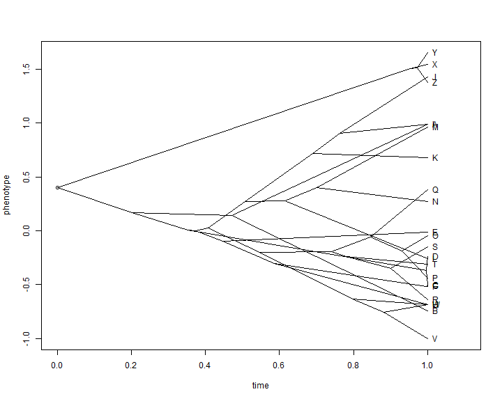
This is not super pretty, and we can do much better with canned routines that also allow us to automatically space the labels of tip taxa on the tree:
phenogram(tree, x, spread.labels = TRUE)
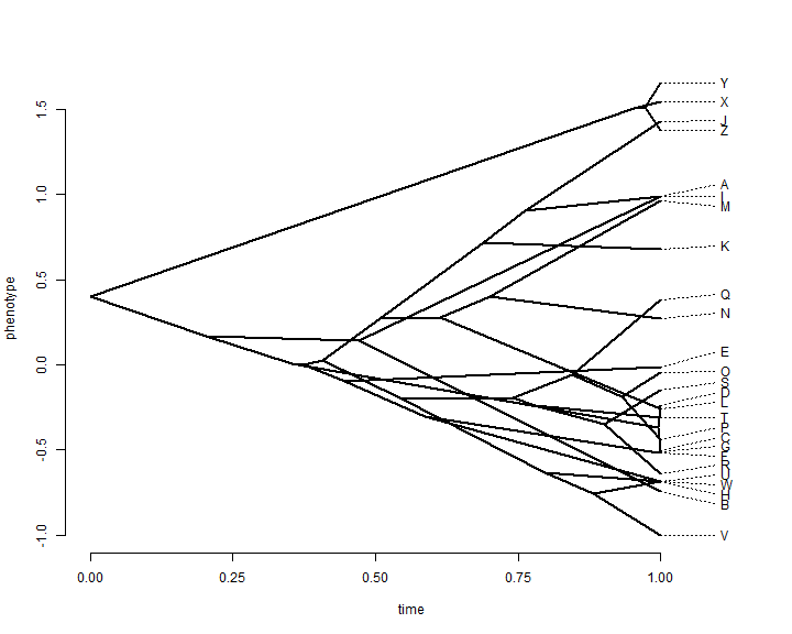
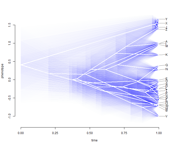
This plot throws out all the information that we have about uncertainty in
reconstructed ancestral trait values. "phytools" has a function which
overlays a 95% confidence limit using transparency. Here is a demo of what that looks
like:
fancyTree(tree, type = "phenogram95", x = x)
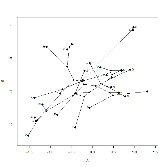
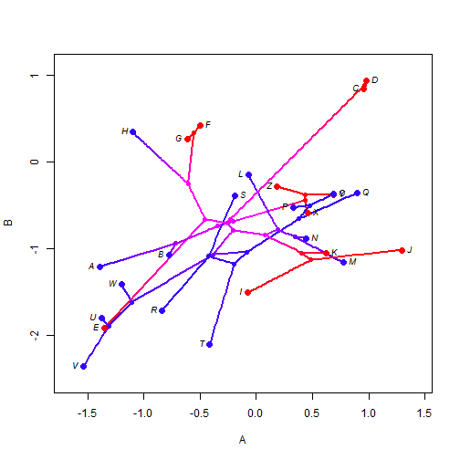
We can also project a tree into a two-trait morphospace. The general approach
for this is simple, but "phytools" has canned routines to
generate this phylomorphospace visualization:
## simulate data with a modest (0.5) correlation
XY <- sim.corrs(tree, vcv = matrix(c(1, 0.5, 0.5, 1), 2, 2))
colnames(XY) <- LETTERS[1:2]
## project into morphospace
phylomorphospace(tree, XY, label = "horizontal")
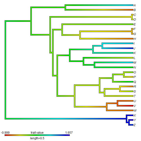
The final type of visualization that we can use with ancestral character
reconstruction for continuous traits uses the function contMap in
phytools which maps the observed and reconstructed phenotypic trait values onto
the tree using a color gradient.
## create contMap
XX <- contMap(tree, x)
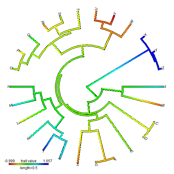
We can also do a circular style tree.
plot(XX, type = "fan")
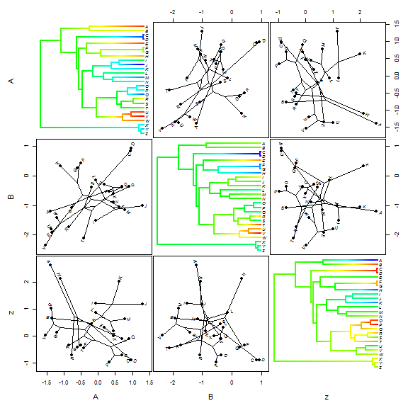
One last thing for visualizing ancestral state values for continuous traits.
"phytools now has a function which can be used to create a
"phylogenetic scattergram" - containing contMap plots on the diagonal and
bivariate projections of the tree into morphospace on off-diagonal positions.
Here is a demo of this function:
## simulate a third character
z <- fastBM(tree, sig2 = 2)
XYZ <- cbind(XY, z)
fancyTree(tree, X = XYZ, type = "scattergram")
Discrete character data - particular whose evolution is modeled by a continuous time Markov chain (i.e., a non-QG model) - are not the focus of this course. However it is nonetheless useful to know how to do this properly in R.
"phytools" has a function for ancestral character estimation under
a couple of different models that uses the re-rooting method of Yang (1995). For
other models of evolutionary change not covered by this function, users should try
Rich Fitzjohn's diversitree
package.
## simulate discrete character data
Q <- matrix(c(-2, 1, 1, 1, -2, 1, 1, 1, -2), 3, 3)
colnames(Q) <- rownames(Q) <- letters[1:3]
x <- sim.history(tree, Q, anc = "a")$states
print(x)
##   Z   Y   X   W   V   U   T   S   R   Q   P   O   N   M   L   K   J   I
## "b" "b" "b" "a" "a" "c" "c" "a" "a" "a" "a" "a" "c" "c" "a" "b" "b" "b"
##   H   G   F   E   D   C   B   A
## "a" "b" "b" "b" "b" "b" "c" "a"
## estimate ancestral states under a ER model
fitER <- rerootingMethod(tree, x, model = "ER")
print(fitER)
## $loglik
## [1] -21
##
## $Q
##         a       b       c
## a -1.7772  0.8886  0.8886
## b  0.8886 -1.7772  0.8886
## c  0.8886  0.8886 -1.7772
##
## $marginal.anc
##            a         b         c
## 27 3.506e-01 0.4098640 2.396e-01
## 28 7.889e-04 0.9984445 7.665e-04
## 29 3.833e-05 0.9999241 3.758e-05
## 30 3.965e-01 0.4042201 1.993e-01
## 31 4.081e-01 0.4728409 1.190e-01
## 32 4.192e-01 0.4703570 1.105e-01
## 33 4.482e-01 0.4365387 1.153e-01
## 34 7.674e-01 0.1481032 8.449e-02
## 35 8.773e-01 0.0315238 9.117e-02
## 36 8.228e-01 0.0206660 1.565e-01
## 37 9.437e-01 0.0167132 3.956e-02
## 38 9.267e-01 0.0157189 5.755e-02
## 39 9.927e-01 0.0023788 4.894e-03
## 40 9.909e-01 0.0033804 5.673e-03
## 41 9.989e-01 0.0004878 5.868e-04
## 42 3.361e-01 0.4845388 1.793e-01
## 43 3.439e-01 0.2750909 3.810e-01
## 44 1.811e-01 0.1502825 6.686e-01
## 45 6.565e-02 0.8908456 4.350e-02
## 46 3.207e-02 0.9445953 2.334e-02
## 47 3.854e-01 0.5102367 1.043e-01
## 48 4.019e-01 0.4955680 1.026e-01
## 49 1.772e-05 0.9999707 1.158e-05
## 50 1.283e-05 0.9999766 1.057e-05
## 51 4.243e-01 0.2565491 3.192e-01
Now let's plot estimated marginal ancestral states on the tree.
plotTree(tree, setEnv = TRUE, offset = 0.5)
## setEnv=TRUE is experimental. please be patient with bugs
nodelabels(node = as.numeric(rownames(fitER$marginal.anc)), pie = fitER$marginal.anc,
    piecol = c("blue", "red", "yellow"), cex = 0.6)
tiplabels(pie = to.matrix(x, sort(unique(x))), piecol = c("blue", "red", "yellow"),
    cex = 0.3)
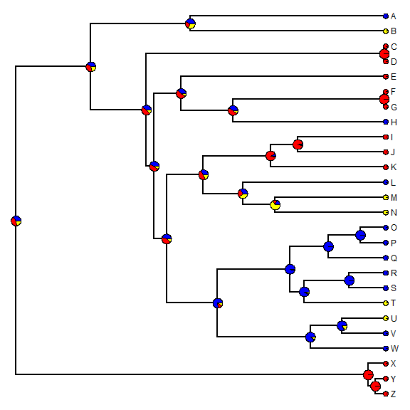
An alternative approach to the one outline above is to use an MCMC approach to sample character histories from their posterior probability distribution. This is called stochastic character mapping (Huelsenbeck et al. 2003). The model is the same but in this case we get a sample of unambiguous histories for our discrete character's evolution on the tree - rather than a probability distribution for the character at nodes.
For instance, given the data simulated above - we can generate the stochastic character map as follows:
## simulate single stochastic character map using empirical Bayes method
mtree <- make.simmap(tree, x, model = "ER")
##         a       b       c
## a -1.7772  0.8886  0.8886
## b  0.8886 -1.7772  0.8886
## c  0.8886  0.8886 -1.7772
##      a      b      c
## 0.3333 0.3333 0.3333
cols <- setNames(c("blue", "red", "yellow"), sort(unique(x)))
plotSimmap(mtree, cols, pts = FALSE, lwd = 3)
add.simmap.legend(colors = cols, vertical = FALSE, prompt = FALSE, x = 0, y = 24)
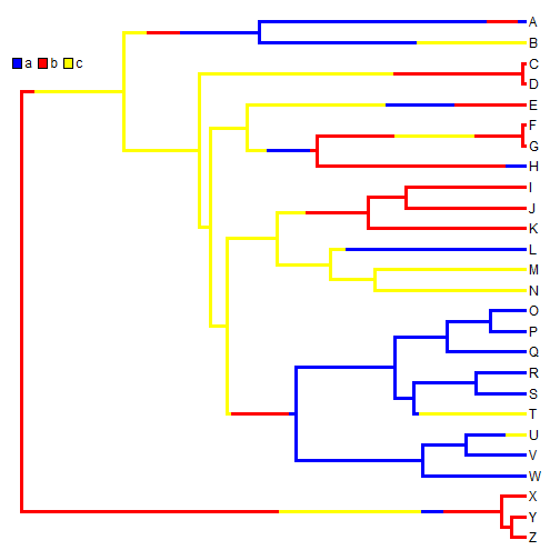
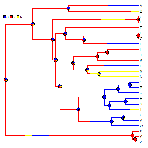
A single stochastic character map does not mean a whole lot in isolation; however in aggregate, we can do quite a bit. For instance, we can estimate the number of changes of each type, the proportion of time spent in each state, and the posterior probabilities that each internal node is in each state, under our model. For example:
## simulate 200 stochastic character maps
mtrees <- make.simmap(tree, x, model = "ER", nsim = 200)
##         a       b       c
## a -1.7772  0.8886  0.8886
## b  0.8886 -1.7772  0.8886
## c  0.8886  0.8886 -1.7772
##      a      b      c
## 0.3333 0.3333 0.3333
XX <- describe.simmap(mtrees, plot = FALSE)
## 200 trees with a mapped discrete character with states:
##  a, b, c
##
## trees have 18.785 changes between states on average
##
## changes are of the following types:
##       a,b   a,c   b,a   b,c  c,a  c,b
## x->y 3.89 4.365 3.115 2.515 2.58 2.32
##
## mean total time spent in each state is:
##           a     b      c total
## raw  4.0828 3.571 1.8944 9.548
## prop 0.4276 0.374 0.1984 1.000
## now let's plot a random map, and overlay the posterior probabilities
plotSimmap(mtrees[[1]], cols, lwd = 3, pts = F, setEnv = T)
## setEnv=TRUE is experimental. please be patient with bugs
nodelabels(pie = XX$ace, piecol = cols, cex = 0.6)
add.simmap.legend(colors = cols, vertical = FALSE, prompt = FALSE, x = 0, y = 24)
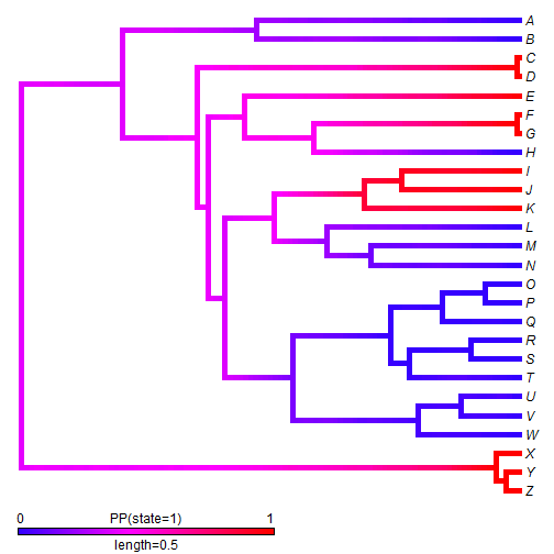
We can also use stochastic mapping to plot the posterior probability that the edges & nodes of the tree are in a binary state. This function is somewhat primitive, so we first have to convert our mapped edge states to 0 & 1.
## convert mapped states
stateb <- mergeMappedStates(mtrees, c("a", "c"), "0")
stateb <- mergeMappedStates(stateb, "b", "1")
## now plot density map
XX <- densityMap(stateb, lwd = 5)
Discrete & continuous character visualizations can be combined in a range of ways. For instance, we can overlay a density map onto a phylomorphospace plot, as follows:
phylomorphospace(XX$tree, XY, label = "horizontal", colors = XX$cols, node.by.map = TRUE)
That's all for now!
Written by Liam J. Revell. Last updated Aug. 6, 2013