t <- 0:100  # time
sig2 <- 0.01
## first, simulate a set of random deviates
x <- rnorm(n = length(t) - 1, sd = sqrt(sig2))
## now compute their cumulative sum
x <- c(0, cumsum(x))
plot(t, x, type = "l", ylim = c(-2, 2))
This short tutorial gives some simple approaches that can be used to simulate Brownian evolution in continuous and discrete time, in the absence of and on a tree.
Brownian motion is a stochastic model in which changes from one time to the next are random draws from a normal distribution with mean 0.0 and variance σ2 × Δt. In other words, the expected variance under Brownian motion increases linearly through time with instantaneous rate σ2.
Before we begin, to the extent that you would like to try and follow along, it's
probably wise to download & install the latest version of my package,
"phytools". You could download the source or an appropriate compiled
package binary from here:
http://www.phytools.org/eqg/phytools/.
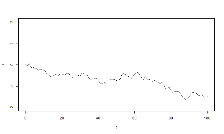
Brownian motion is very easy to simulate. To start off, let's simulate a single instance of Brownian motion for 100 generations of discrete time in which the variance of the diffusion process is σ2 = 0.01 per generation.
t <- 0:100 # time sig2 <- 0.01 ## first, simulate a set of random deviates x <- rnorm(n = length(t) - 1, sd = sqrt(sig2)) ## now compute their cumulative sum x <- c(0, cumsum(x)) plot(t, x, type = "l", ylim = c(-2, 2))

The trick here is that we draw random normal deviates for the change over each
t time intervals; and then to get the state of our chain at each time
interval we just compute the cumulative sum of all the individual changes
using cumsum. We can do this because the distribution of the changes
under Brownian motion is invariant and does not depend on the state of the
chain.
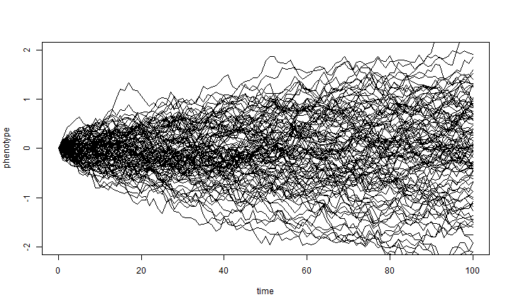
We can also easily do a whole bunch of simulations like this at once, using the same conditions:
nsim <- 100
X <- matrix(rnorm(n = nsim * (length(t) - 1), sd = sqrt(sig2)), nsim, length(t) -
    1)
X <- cbind(rep(0, nsim), t(apply(X, 1, cumsum)))
plot(t, X[1, ], xlab = "time", ylab = "phenotype", ylim = c(-2, 2), type = "l")
apply(X[2:nsim, ], 1, function(x, t) lines(t, x), t = t)
## NULL
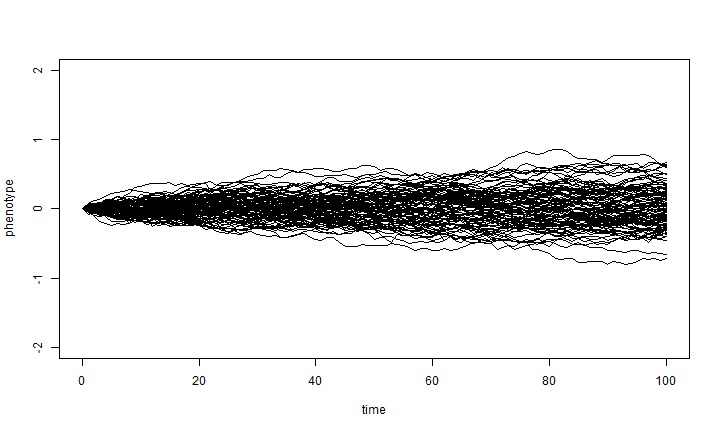
To see how the outcome depends on σ2, let's compate the result
when we divide sig2 by 10:
X <- matrix(rnorm(n = nsim * (length(t) - 1), sd = sqrt(sig2/10)), nsim, length(t) -
    1)
X <- cbind(rep(0, nsim), t(apply(X, 1, cumsum)))
plot(t, X[1, ], xlab = "time", ylab = "phenotype", ylim = c(-2, 2), type = "l")
apply(X[2:nsim, ], 1, function(x, t) lines(t, x), t = t)
## NULL
Cool.
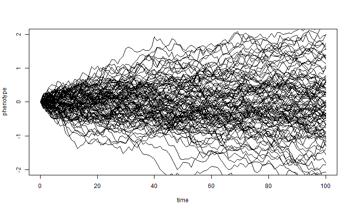
There are a number of different ways we could've done this. For example, instead
of using apply, which economizes on code, we could have used a
for loop as follows:
X <- matrix(0, nsim, length(t))
for (i in 1:nsim) X[i, ] <- c(0, cumsum(rnorm(n = length(t) - 1, sd = sqrt(sig2))))
plot(t, X[1, ], xlab = "time", ylab = "phenotype", ylim = c(-2, 2), type = "l")
for (i in 1:nsim) lines(t, X[i, ])
As mentioned above, the expected variance under Brownian motion is just σ2 × t. To see this easiest, we can just do the following. Here I will use 10,000 simulations for 100 generations under the same conditions to "smooth out" our result:
nsim <- 10000
X <- matrix(rnorm(n = nsim * (length(t) - 1), sd = sqrt(sig2)), nsim, length(t) -
    1)
X <- cbind(rep(0, nsim), t(apply(X, 1, cumsum)))
v <- apply(X, 2, var)
plot(t, v, type = "l", xlab = "time", ylab = "variance among simulations")
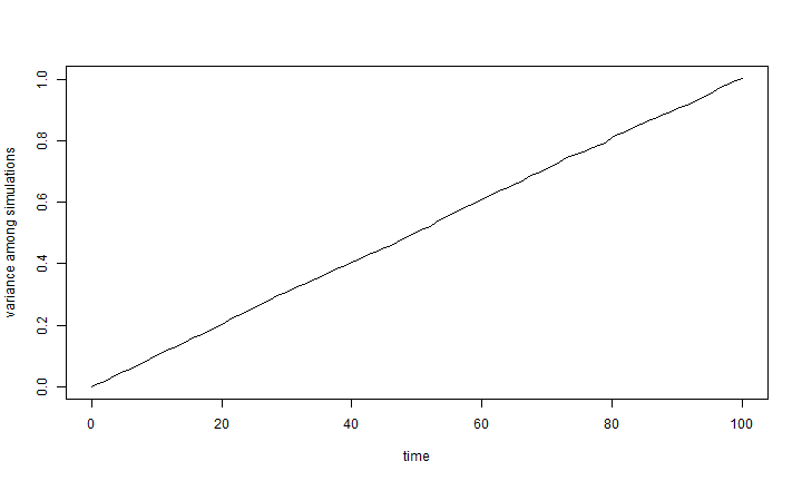
var(X[, length(t)]) # this should be about 1.00
## [1] 1.003
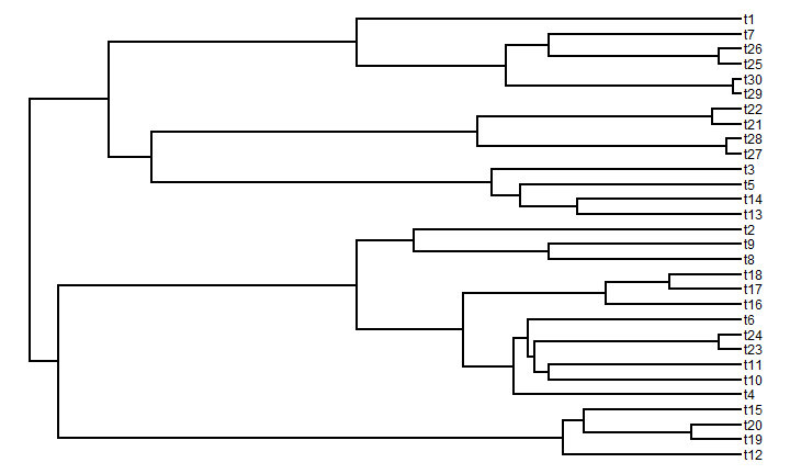
OK, now let's try to simulate using Brownian motion up the branches of a tree.
Sticking with discrete time, we first need a discrete time phylogeny, which we can
simulate using pbtree in the "phytools" package:
library(phytools)
t <- 100  # total time
n <- 30  # total taxa
b <- (log(n) - log(2))/t
tree <- pbtree(b = b, n = n, t = t, type = "discrete")
## simulating with both taxa-stop (n) and time-stop (t) is
## performed via rejection sampling & may be slow
##
##   31 trees rejected before finding a tree
plotTree(tree)
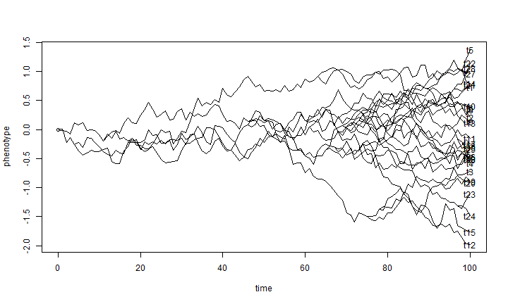
Now, to simulate on all the branches of the tree we just need to simulate on each branch separately, and then "shift" each daughter branch by the end state of it's parent. We can do this, remember, because the outcome of Brownian evolution at each time step is independent of all other time steps.
## simulate evolution along each edge
X <- lapply(tree$edge.length, function(x) c(0, cumsum(rnorm(n = x, sd = sqrt(sig2)))))
## reorder the edges of the tree for pre-order traversal
cw <- reorder(tree)
## now simulate on the tree
ll <- tree$edge.length + 1
for (i in 1:nrow(cw$edge)) {
    pp <- which(cw$edge[, 2] == cw$edge[i, 1])
    if (length(pp) > 0)
        X[[i]] <- X[[i]] + X[[pp]][ll[pp]] else X[[i]] <- X[[i]] + X[[1]][1]
}
## get the starting and ending points of each edge for plotting
H <- nodeHeights(tree)
## plot the simulation
plot(H[1, 1], X[[1]][1], ylim = range(X), xlim = range(H), xlab = "time", ylab = "phenotype")
for (i in 1:length(X)) lines(H[i, 1]:H[i, 2], X[[i]])
## add tip labels if desired
yy <- sapply(1:length(tree$tip.label), function(x, y) which(x == y), y = tree$edge[,
    2])
yy <- sapply(yy, function(x, y) y[[x]][length(y[[x]])], y = X)
text(x = max(H), y = yy, tree$tip.label)
There are probably many more economical ways to do that, but this is one.
In reality, most simulations of Brownian motion are conducted using continuous rather than discrete time. This is because the additivity of Brownian motion means that the expected variances among & covariances between species are the same in whether we simulate t steps each with variance σ2, or one big step with variance σ2t.
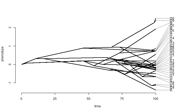
Here is an example of a continuous time simulation & visualization using canned functions.
## simulate Brownian evolution on a tree with fastBM
x <- fastBM(tree, sig2 = sig2, internal = TRUE)
## visualize Brownian evolution on a tree
phenogram(tree, x, spread.labels = TRUE, spread.cost = c(1, 0))
A few additional points about Brownian evolution were made by Joe in his lecture on the topic, so I have added some additional simulations to illustrate these points.
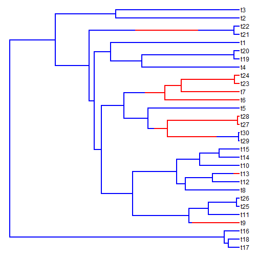
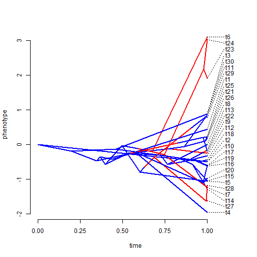
Joe pointed out that in some cases there might be different rates of Brownian evolution in different parts of the tree. It is straightforward to simulate Brownian motion with different rates on different branches. For example, in the following example, I first simulate the history of a discretely valued character on the tree, and then a continuous trait with a rate that changes as a function of the mapped discrete character. I'll then create a traitgram that projects the phylogeny onto the phenotypic trait axis and overlays the mapped discrete character.
set.seed(100)
## transition matrix for the discrete trait simulation
Q <- matrix(c(-1, 1, 1, -1), 2, 2)
## simulated tree
tree <- pbtree(n = 30, scale = 1)
## simulate discrete character history
tree <- sim.history(tree, Q, anc = "1")
## plot discrete character history on the tree
plotSimmap(tree, setNames(c("blue", "red"), 1:2), pts = F)
x <- sim.rates(tree, setNames(c(1, 20), 1:2), internal = TRUE)
phenogram(tree, x, colors = setNames(c("blue", "red"), 1:2), spread.labels = TRUE,
    spread.cost = c(1, 0))
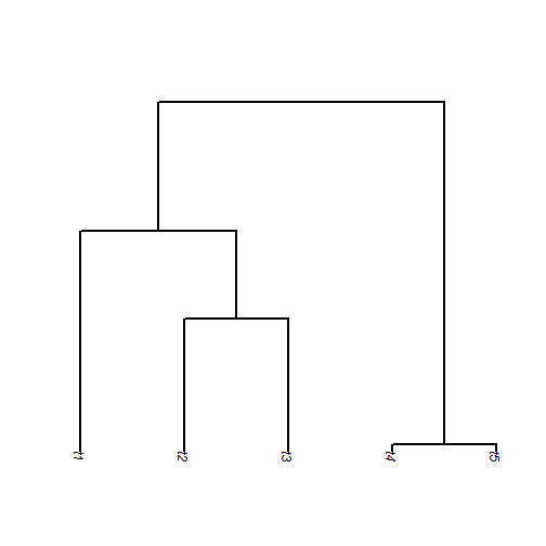
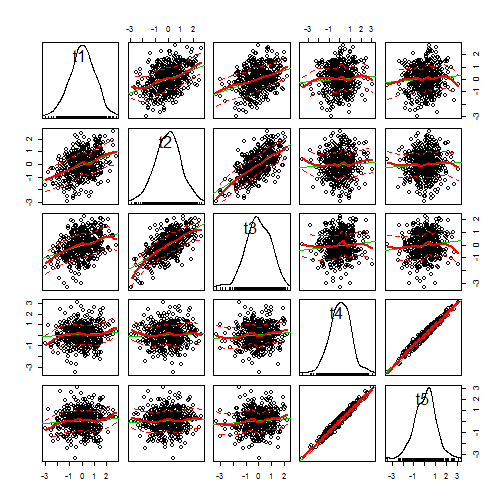
Joe discussed the fact that shared ancestry creates "covariance"
among the tips of the tree. In my presentation, I described how this
is equivalent to covariance among species across a large number of
replications of the evolutionary process. The following is an
illustration of that point. (This requires the package
"car".)
## simulate 5 taxon tree
tree <- pbtree(n = 5)
## 500 BM simulations
X <- fastBM(tree, nsim = 500)
## plot tree
plot(tree, edge.width = 2, direction = "downwards")
## plot distribution across tips from 500 simulations
require(car)
scatterplotMatrix(t(X))
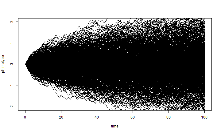
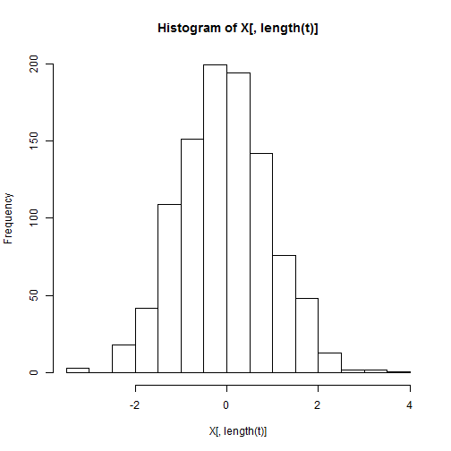
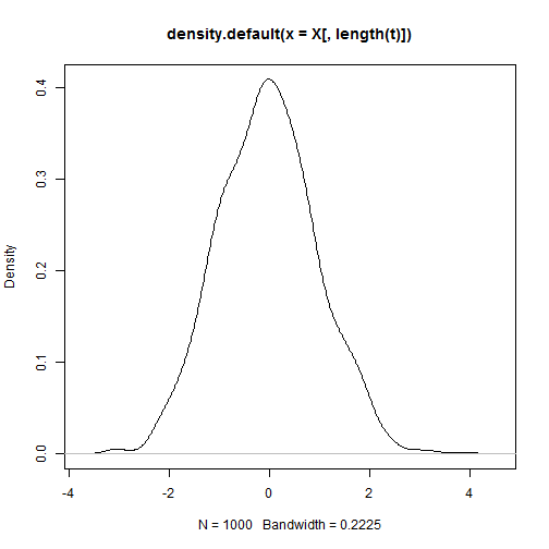
Joe pointed out that Brownian motion does not assume that the process under which the individual lineages are moving is Gaussian. The result will be Gaussian - due to the Central Limit Theorem. Here is an illustration of that:
t <- 0:100  # time
sig2 <- 0.01
nsim <- 1000
## we'll simulate the steps from a uniform distribution with limits set to
## have the same variance (0.01) as before
X <- matrix(runif(n = nsim * (length(t) - 1), min = -sqrt(3 * sig2), max = sqrt(3 *
    sig2)), nsim, length(t) - 1)
X <- cbind(rep(0, nsim), t(apply(X, 1, cumsum)))
plot(t, X[1, ], xlab = "time", ylab = "phenotype", ylim = c(-2, 2), type = "l")
apply(X[2:nsim, ], 1, function(x, t) lines(t, x), t = t)
## NULL
var(X[, length(t)])
## [1] 0.969
hist(X[, length(t)])
plot(density(X[, length(t)]))
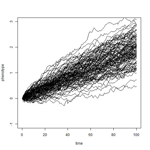
Thomas pointed out that Brownian motion is generally assumed to be trendless; however it is possible to simulate and (under some conditions) fit a model of Brownian evolution with a trend. Here is an example of a simulation (using the same general approach as above) with a trend.
nsim = 100
X <- matrix(rnorm(mean = 0.02, n = nsim * (length(t) - 1), sd = sqrt(sig2/4)),
    nsim, length(t) - 1)
X <- cbind(rep(0, nsim), t(apply(X, 1, cumsum)))
plot(t, X[1, ], xlab = "time", ylab = "phenotype", ylim = c(-1, 3), type = "l")
apply(X[2:nsim, ], 1, function(x, t) lines(t, x), t = t)
## NULL
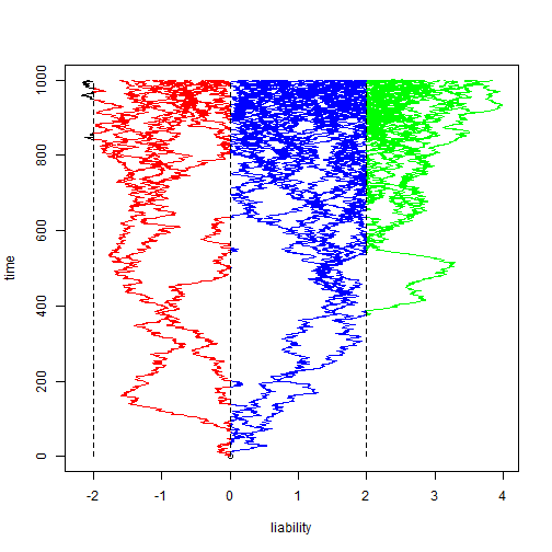
Finally, Joe mentioned the threshold model - so I'm obligated to show
that "phytools" can do simulation and plotting under the
threshold model. Here is an example:
tree <- pbtree(n = 100, scale = 1)
xx <- bmPlot(tree, sig2 = 2/1000, type = "threshold", thresholds = c(-2, 0,
    2))
That's it!
Written by Liam J. Revell. Last updated Aug. 8, 2013