## first load phytools
require(phytools)
## simulate a tree
tree <- pbtree(n = 26, tip.label = LETTERS)
plotTree(tree)
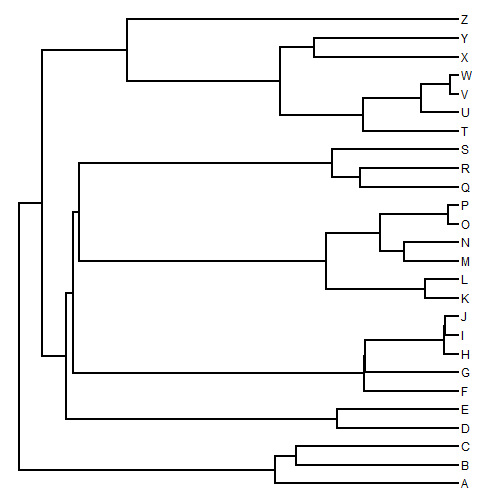
In this tutorial I'm going to quickly overview a range of plotting methods for phylogenies & comparative data that are implemented in the phytools package.
The first plotting method I'll illustrate is called a 'traitgram' which is a projection of the tree into a space defined by trait values & time since the root. So, for example:
## first load phytools require(phytools) ## simulate a tree tree <- pbtree(n = 26, tip.label = LETTERS) plotTree(tree)

## simulate data under Brownian motion
x <- fastBM(tree)
x
##        A        B        C        D        E        F        G        H
##  2.21950  0.25627  1.94721 -1.85028 -1.08259  0.64343  0.51627  1.29706
##        I        J        K        L        M        N        O        P
##  0.95156  1.76106 -1.51259 -1.43161  0.67923  1.23026  0.94695  1.02401
##        Q        R        S        T        U        V        W        X
##  0.52726  0.70021  0.51362  0.17891  0.28827  0.66855  0.75961  0.07452
##        Y        Z
## -0.19691  0.24588
## plot a simple traitgram
phenogram(tree, x)
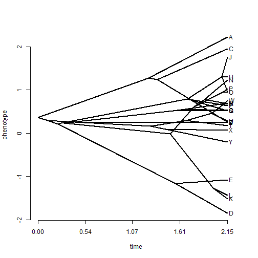
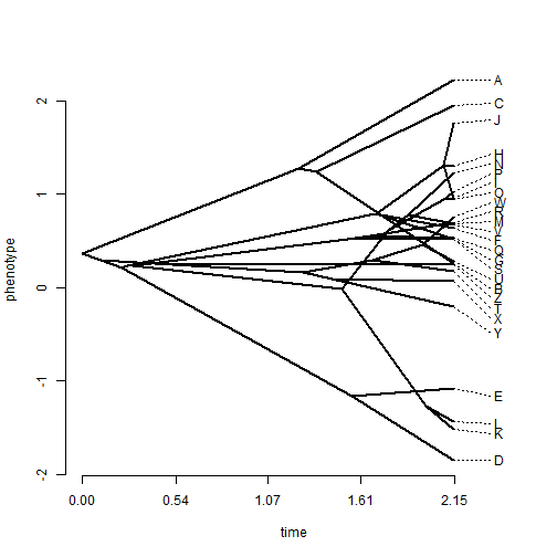
## tip labels are messy - spread them
phenogram(tree, x, spread.labels = TRUE)
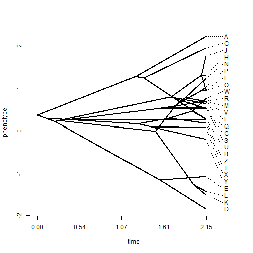
## change the spread costs
phenogram(tree, x, spread.labels = TRUE, spread.cost = c(1, 0))
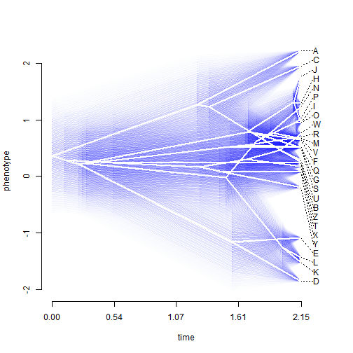
We can also plot a traitgram with the uncertainty about ancestral character states visualized using transparent probability density. This is implemented in the phytools function fancyTree. So, for instance:
## plot traitgram with 95% CI
fancyTree(tree, type = "phenogram95", x = x, spread.cost = c(1, 0))
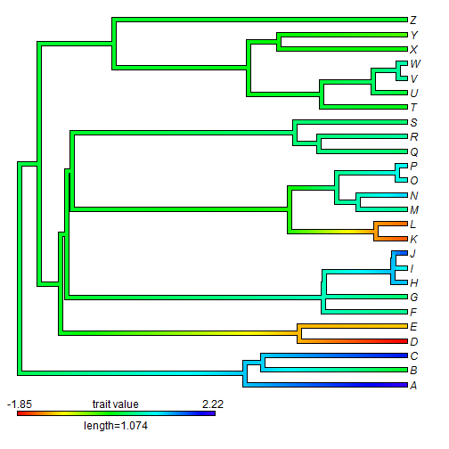
Next, we can explore the continuous character mapping function in phytools called contMap. Here is a quick demo using the same data:
## plot contMap
obj <- contMap(tree, x)
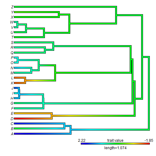
contMap returns an object of class "contMap" which we can then more easily replot using, for instance, different parameters:
## plot leftward
plot(obj, direction = "leftwards")
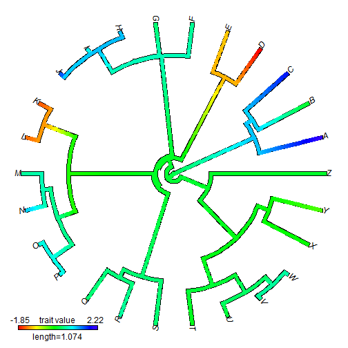
## plot fan style tree
plot(obj, type = "fan", lwd = 5)  ## for example
Here are some real data using anole.tre and svl.csv:
anole.tree <- read.tree("anole.tre")
## or
## anole.tree<-read.tree('http://www.phytools.org/anthrotree/plot/anole.tre')
anole.tree
##
## Phylogenetic tree with 100 tips and 99 internal nodes.
##
## Tip labels:
## 	ahli, allogus, rubribarbus, imias, sagrei, bremeri, ...
##
## Rooted; includes branch lengths.
svl <- read.csv("svl.csv", header = TRUE, row.names = 1)
## of
## svl<-read.csv('http://www.phytools.org/anthrotree/plot/svl.csv',header=TRUE,row.names=1)
svl <- as.matrix(svl)[, 1]
svl
##            ahli         alayoni         alfaroi        aliniger
##           4.039           3.816           3.527           4.037
##        allisoni         allogus   altitudinalis         alumina
##           4.375           4.040           3.843           3.589
##       alutaceus     angusticeps     argenteolus     argillaceus
##           3.555           3.789           3.971           3.758
##         armouri   bahorucoensis        baleatus        baracoae
##           4.122           3.827           5.053           5.043
##       barahonae        barbatus        barbouri        bartschi
##           5.077           5.004           3.664           4.281
##         bremeri        breslini    brevirostris        caudalis
##           4.113           4.051           3.874           3.912
##       centralis  chamaeleonides    chlorocyanus     christophei
##           3.698           5.042           4.275           3.885
##       clivicola     coelestinus        confusus           cooki
##           3.759           4.298           3.938           4.092
##    cristatellus    cupeyalensis         cuvieri    cyanopleurus
##           4.190           3.462           4.875           3.630
##         cybotes     darlingtoni       distichus dolichocephalus
##           4.211           4.302           3.929           3.909
##       equestris      etheridgei   eugenegrahami       evermanni
##           5.114           3.658           4.129           4.166
##         fowleri         garmani         grahami           guafe
##           4.289           4.769           4.154           3.877
##       guamuhaya         guazuma       gundlachi       haetianus
##           5.037           3.764           4.188           4.317
##      hendersoni      homolechis           imias    inexpectatus
##           3.860           4.033           4.100           3.537
##       insolitus        isolepis           jubar           krugi
##           3.800           3.657           3.953           3.887
##      lineatopus   longitibialis        loysiana          lucius
##           4.129           4.242           3.701           4.199
##    luteogularis      macilentus        marcanoi          marron
##           5.101           3.716           4.079           3.832
##         mestrei       monticola          noblei        occultus
##           3.987           3.771           5.083           3.663
##         olssoni        opalinus      ophiolepis        oporinus
##           3.794           3.838           3.638           3.846
##        paternus        placidus       poncensis        porcatus
##           3.803           3.774           3.820           4.259
##          porcus      pulchellus         pumilis quadriocellifer
##           5.038           3.799           3.467           3.902
##      reconditus        ricordii     rubribarbus          sagrei
##           4.483           5.014           4.078           4.067
##    semilineatus        sheplani         shrevei      singularis
##           3.697           3.683           3.983           4.058
##      smallwoodi         strahmi       stratulus     valencienni
##           5.035           4.274           3.870           4.322
##       vanidicus    vermiculatus        websteri       whitemani
##           3.626           4.803           3.917           4.097
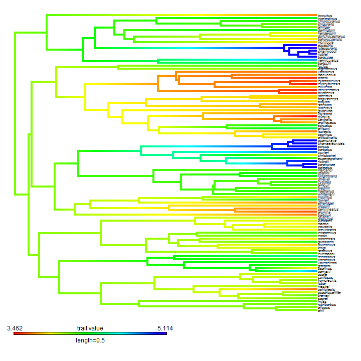
obj <- contMap(anole.tree, svl, fsize = c(0.6, 1), outline = FALSE)
We can also plot this using a circular or fan tree:
plot(obj, type = "fan", outline = FALSE)
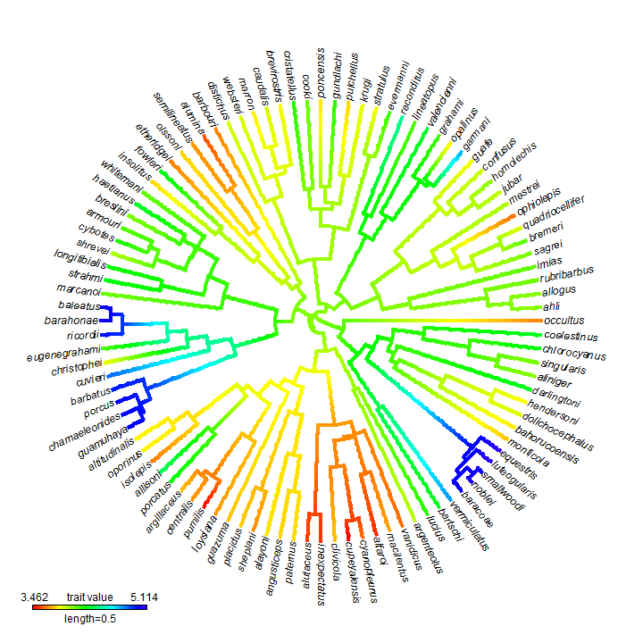
Note that the intense aliasing is just a byproduct of plotting to .png format. To get a high quality image we can plot to .pdf or other formats. For instance:
pdf(file = "anole.contMap.pdf", width = 10, height = 10)
plot(obj, type = "fan", outline = FALSE)
dev.off()
## pdf
##   2
The result can be viewed here.
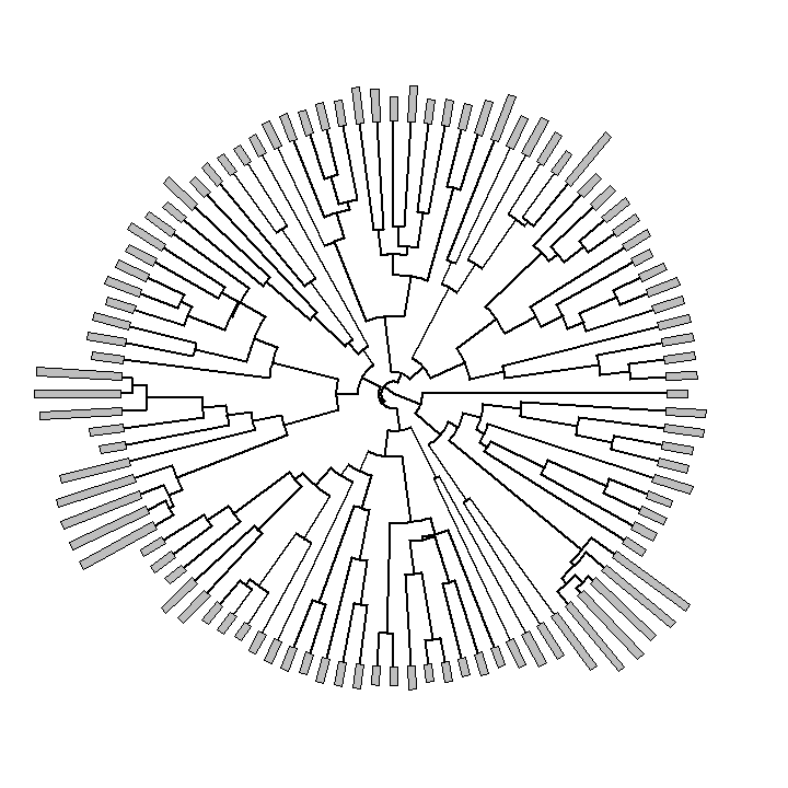
Finally, a relatively simple new plotting method in phytools is the function plotTree.wBars. This function is not in the current CRAN release of phytools, so to run it you will need to first download & install phytools from source. That function pretty much does what it sounds like it does:
plotTree.wBars(anole.tree, exp(svl), type = "fan", scale = 0.002)
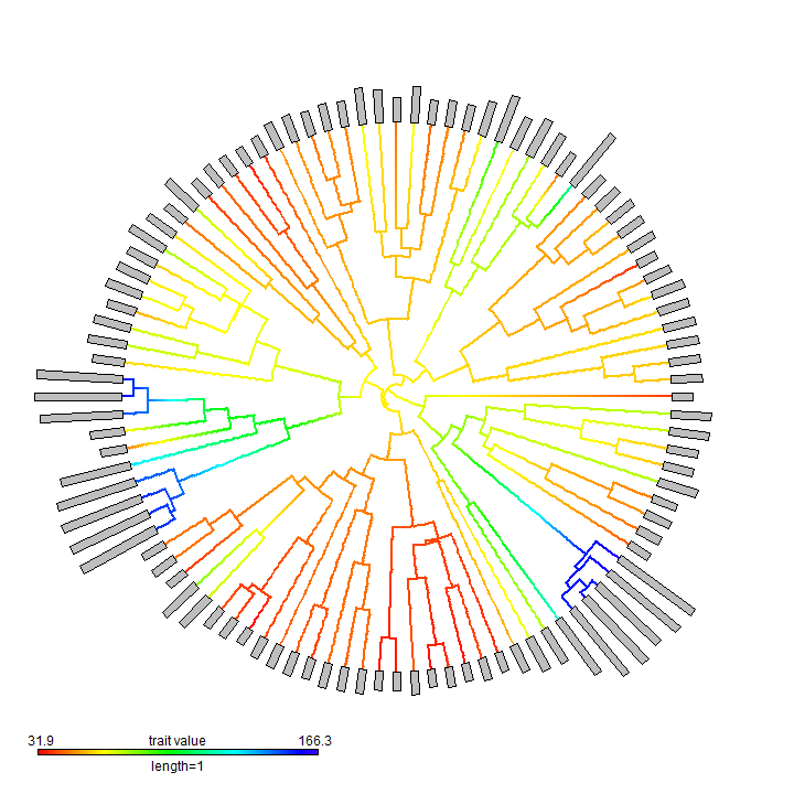
This is also kind of cool:
obj <- contMap(anole.tree, exp(svl), plot = FALSE)
plotTree.wBars(obj$tree, exp(svl), method = "plotSimmap", colors = obj$cols,
    type = "fan", scale = 0.002)
add.color.bar(1, obj$cols, title = "trait value", lims = obj$lims, prompt = FALSE,
    x = 0.9 * par()$usr[1], y = 0.9 * par()$usr[3])
pdf(file = "anole.plotTree.wBars.pdf", width = 10, height = 10)
plotTree.wBars(obj$tree, exp(svl), method = "plotSimmap", colors = obj$cols,
    type = "fan", scale = 0.002)
add.color.bar(1, obj$cols, title = "trait value", lims = obj$lims, prompt = FALSE,
    x = 0.9 * par()$usr[1], y = 0.9 * par()$usr[3])
dev.off()
## pdf
##   2
(A non-aliased version here.)
We can also do two dimensional visualizations of phylogenies in morphospace. The is called a 'phylomorphospace'. E.g.:
X <- fastBM(tree, nsim = 3)  ## simulate 3 characters
phylomorphospace(tree, X[, c(1, 2)], xlab = "trait 1", ylab = "trait 2")
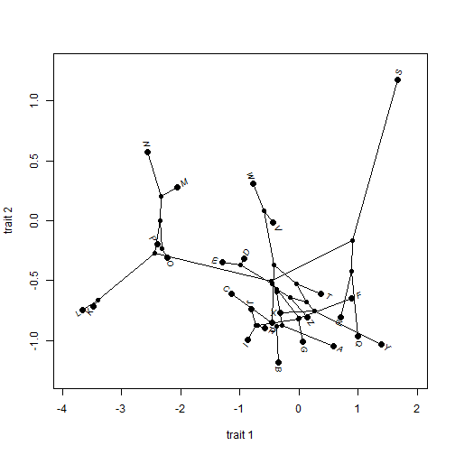
With phytools we can do static or animated version of the same. I'll just do a static version here, but animated is the default:
phylomorphospace3d(tree, X, method = "static")
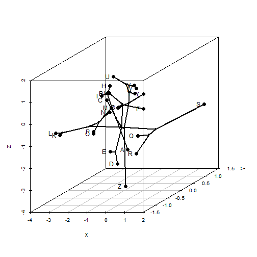
Try the animated version on your own.
Finally, it's possible to combine the continuous character mapping and 2D phylomorphospaces using a type of phylogenetic scatterplot. Here's a demo:
fancyTree(tree, type = "scattergram", X = X)
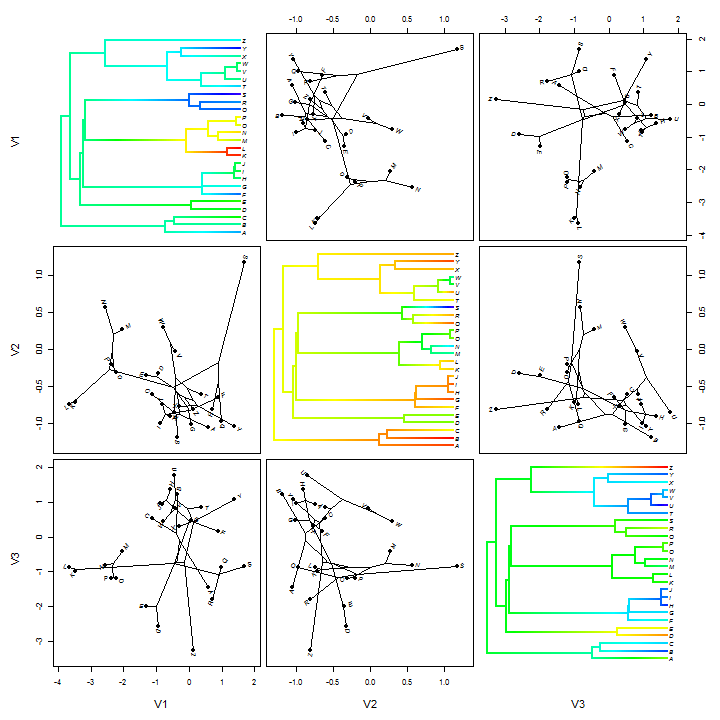
Stochastic character maps are easy to plot using phytools. For instance:
data(anoletree)
plotSimmap(anoletree, type = "fan")
## no colors provided. using the following legend:
##        CG        GB        TC        TG        Tr        Tw
##   "black"     "red"  "green3"    "blue"    "cyan" "magenta"
## setEnv=TRUE for this type is experimental. please be patient with bugs
## we can use any color scheme, but this is the default
cols <- setNames(palette()[1:length(unique(getStates(anoletree, "tips")))],
    sort(unique(getStates(anoletree, "tips"))))
add.simmap.legend(colors = cols, x = 0.9 * par()$usr[1], y = 0.9 * par()$usr[4],
    prompt = FALSE)
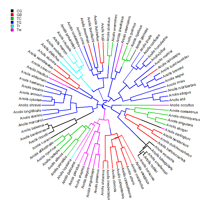
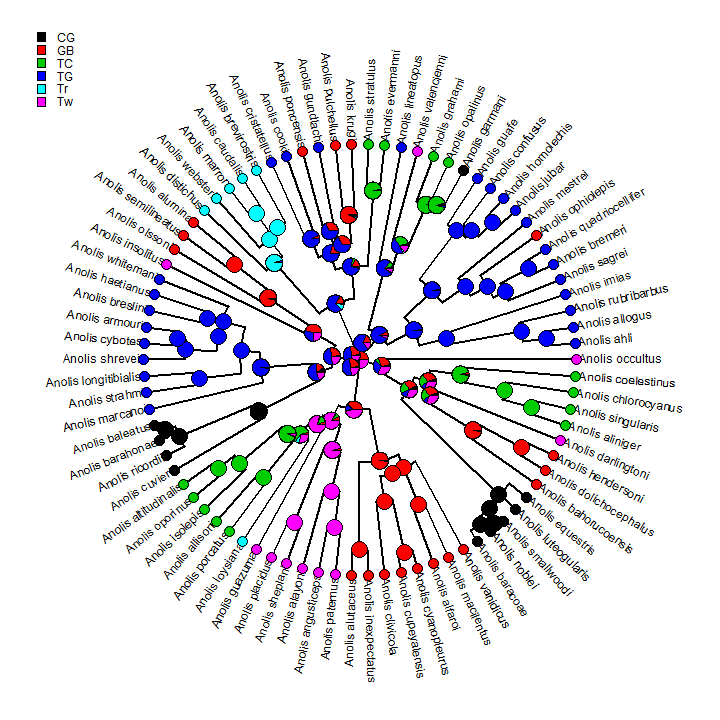
This is just one stochastically mapped tree. Let's perform the method of stochastic mapping & plot the posterior probabilities at internal nodes.
x <- getStates(anoletree, "tips")
trees <- make.simmap(anoletree, x, model = "ER", nsim = 100)
##          CG       GB       TC       TG       Tr       Tw
## CG -0.11571  0.02314  0.02314  0.02314  0.02314  0.02314
## GB  0.02314 -0.11571  0.02314  0.02314  0.02314  0.02314
## TC  0.02314  0.02314 -0.11571  0.02314  0.02314  0.02314
## TG  0.02314  0.02314  0.02314 -0.11571  0.02314  0.02314
## Tr  0.02314  0.02314  0.02314  0.02314 -0.11571  0.02314
## Tw  0.02314  0.02314  0.02314  0.02314  0.02314 -0.11571
##     CG     GB     TC     TG     Tr     Tw
## 0.1667 0.1667 0.1667 0.1667 0.1667 0.1667
obj <- describe.simmap(trees, plot = FALSE)
obj
## 100 trees with a mapped discrete character with states:
##  CG, GB, TC, TG, Tr, Tw
##
## trees have 25.59 changes between states on average
##
## changes are of the following types:
##      CG,GB CG,TC CG,TG CG,Tr CG,Tw GB,CG GB,TC GB,TG GB,Tr GB,Tw TC,CG
## x->y  0.25  0.31  0.25   0.2  0.32  0.71  1.02   1.2  0.51  1.46  1.25
##      TC,GB TC,TG TC,Tr TC,Tw TG,CG TG,GB TG,TC TG,Tr TG,Tw Tr,CG Tr,GB
## x->y  0.67  0.36  0.69  1.01  1.13  3.25  1.98  1.11  1.66  0.18  0.34
##      Tr,TC Tr,TG Tr,Tw Tw,CG Tw,GB Tw,TC Tw,TG Tw,Tr
## x->y  0.23  0.22  0.45  0.65  1.26  1.49   0.8  0.63
##
## mean total time spent in each state is:
##            CG      GB      TC      TG       Tr      Tw total
## raw  13.09759 46.1139 32.5794 69.7658 12.91992 31.1904 205.7
## prop  0.06368  0.2242  0.1584  0.3392  0.06282  0.1517   1.0
plot(obj, type = "fan")
## setEnv=TRUE for this type is experimental. please be patient with bugs
add.simmap.legend(colors = cols, x = 0.9 * par()$usr[1], y = 0.9 * par()$usr[4],
    prompt = FALSE)
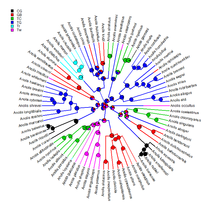
We can also overlay the posterior probabilities on a random stochastic map in a similar way:
plotSimmap(trees[[1]], type = "fan")
## no colors provided. using the following legend:
##        CG        GB        TC        TG        Tr        Tw
##   "black"     "red"  "green3"    "blue"    "cyan" "magenta"
## setEnv=TRUE for this type is experimental. please be patient with bugs
nodelabels(pie = obj$ace, piecol = cols, cex = 0.5)
add.simmap.legend(colors = cols, x = 0.9 * par()$usr[1], y = 0.9 * par()$usr[4],
    prompt = FALSE)
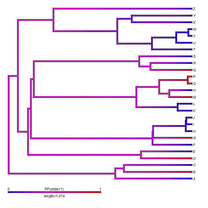
For binary characters, we can also map the posterior density of stochastic maps onto the nodes & branches of a tree using the phytools function densityMap. Here's a demo of this using simulated data.
## first let's simulate data
Q <- matrix(c(-1, 1, 1, -1), 2, 2)
rownames(Q) <- colnames(Q) <- c(0, 1)
tree <- sim.history(tree, Q)
x <- tree$states
x
##   A   B   C   D   E   F   G   H   I   J   K   L   M   N   O   P   Q   R
## "0" "1" "0" "1" "0" "0" "1" "0" "0" "0" "0" "0" "1" "0" "1" "1" "1" "0"
##   S   T   U   V   W   X   Y   Z
## "0" "0" "0" "0" "0" "0" "0" "0"
## stochastic maps
trees <- make.simmap(tree, x, nsim = 100)
##        0      1
## 0 -1.201  1.201
## 1  1.201 -1.201
##   0   1
## 0.5 0.5
## make densityMap
obj <- densityMap(trees, lwd = 4, outline = TRUE)
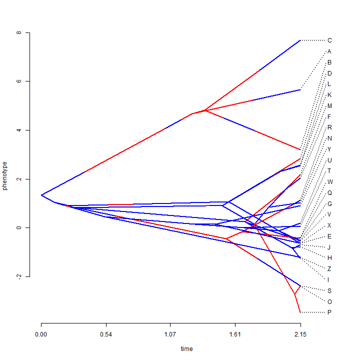
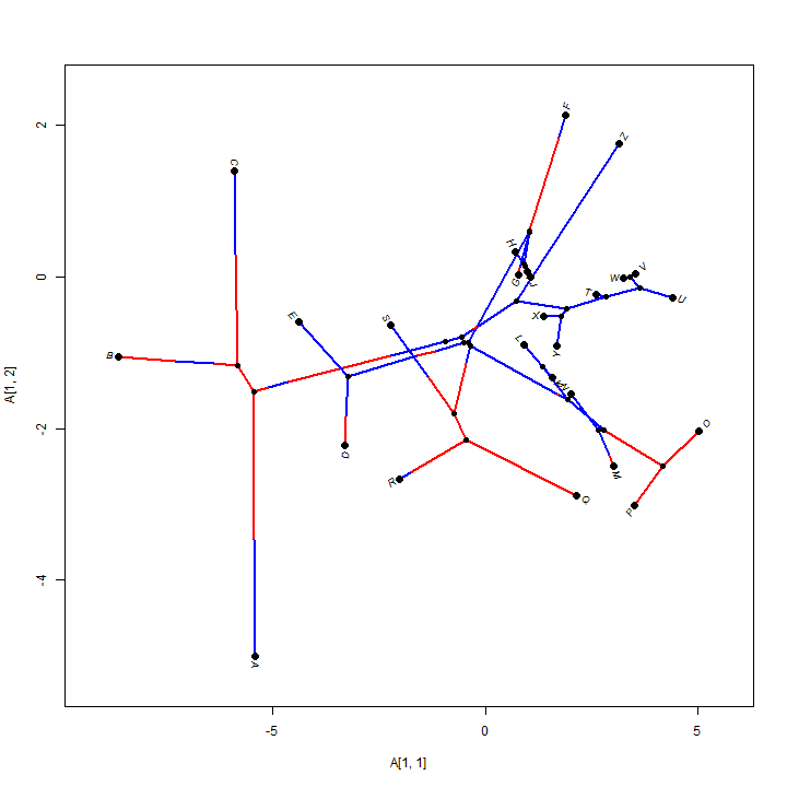
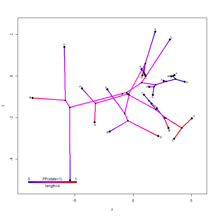
We can, for instance, overlay a discrete character history (or stochastic map) onto a traitgram or phylomorphospace.
## simulate data with a high rate on some branches
x <- sim.rates(tree, setNames(c(1, 10), c(0, 1)))
## plot traitgram
phenogram(tree, x, colors = setNames(c("blue", "red"), c(0, 1)), spread.labels = TRUE,
    spread.cost = c(1, 0))
## we can do the same with phylomorphospaces
X <- cbind(sim.rates(tree, setNames(c(1, 10), c(0, 1))), sim.rates(tree, setNames(c(1,
    10), c(0, 1))))
phylomorphospace(tree, X, colors = setNames(c("blue", "red"), c(0, 1)))
## it is even possible to overlay a posterior density from stochastic mapping
phylomorphospace(obj$tree, X, colors = obj$cols, lwd = 3, xlab = "x", ylab = "y")
add.color.bar(4, obj$cols, title = "PP(state=1)", prompt = FALSE, x = 0.9 *
    par()$usr[1], y = 0.9 * par()$usr[3])
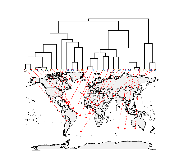
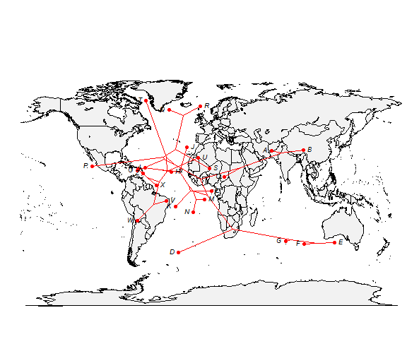
How about projecting a tree onto a geographic map? Here's an example using phytools function phylo.to.map:
# simulate tree & data
tree <- pbtree(n = 26, scale = 100)
tree$tip.label <- LETTERS[26:1]
lat <- fastBM(tree, sig2 = 10, bounds = c(-90, 90))
long <- fastBM(tree, sig2 = 80, bounds = c(-180, 180))
# now plot projection
xx <- phylo.to.map(tree, cbind(lat, long), plot = FALSE)
## tree points to map coordinates
plot(xx, type = "phylogram", asp = 1.3, mar = c(0.1, 0.5, 3.1, 0.1))
## tree projected directly on map
plot(xx, type = "direct", asp = 1.3, mar = c(0.1, 0.5, 3.1, 0.1))
That's all for now!
Written by Liam J. Revell. Last updated May 29, 2014