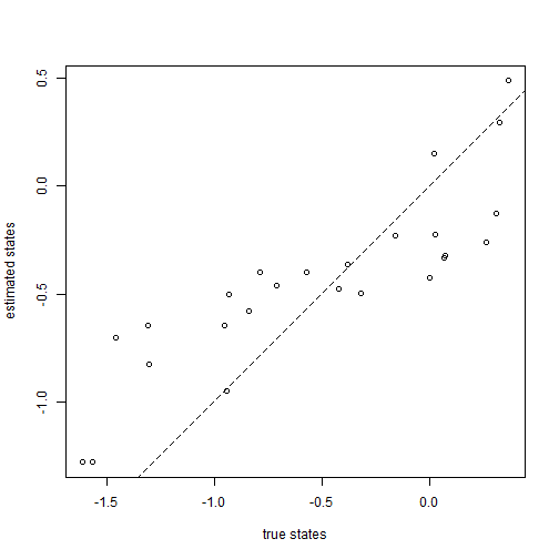
plot(x[1:tree$Nnode + length(tree$tip.label)], fit$par[1:tree$Nnode + 1], xlab = "true states", ylab = "estimated states") lines(range(x), range(x), lty = "dashed") ## 1:1 line
For better or for worse, the estimation of phenotypic trait values for ancestral nodes in the tree continues to be an important goal in phylogenetic comparative biology.
This tutorial focuses on the estimation of ancestral character states under Brownian motion & OU, including when some values for internal nodes are known.
To estimate the states for a continuously valued character at ancestral nodes, we need find the states that have the maximum probability of having arisen under our model. These will be our maximum likelihood estimates.
Since the nodes & tips in the tree have a multivariate normal distribution under Brownian motion, this is relatively simple in principle. We just find the set of parameters & states at internal nodes that maximize the logged, summed multivariate normal density.
## load phytools
library(phytools)
library(mnormt)
## simulate a tree & some data
tree <- pbtree(n = 26, scale = 1)
tree$tip.label <- LETTERS[26:1]
x <- fastBM(tree, internal = TRUE)
## let's try & write down the likelihood function we want
C <- vcvPhylo(tree)
pp <- rep(1, tree$Nnode + 1)
lik <- function(pp, C, x) -sum(dmnorm(c(x, pp[3:length(pp)]), rep(pp[2], nrow(C)),
    pp[1] * C, log = TRUE))
tt <- setNames(c(1, rep(mean(x), tree$Nnode)), c("sig2", 1:tree$Nnode + length(tree$tip)))
fit <- optim(tt, lik, C = C, x = x[1:26], method = "L-BFGS-B", lower = c(1e-06,
    rep(-Inf, tree$Nnode)))
print(fit)
## $par
##    sig2      27      28      29      30      31      32      33      34
##  0.3442 -0.4231 -0.4609 -0.5013 -0.6463 -0.7011 -1.2794 -1.2790 -0.8249
##      35      36      37      38      39      40      41      42      43
## -0.5805 -0.6477 -0.9473 -0.3966  0.1522  0.4888 -0.3975 -0.4942 -0.3624
##      44      45      46      47      48      49      50      51
## -0.4739 -0.3302 -0.3218 -0.2577 -0.1279  0.2937 -0.2226 -0.2300
##
## $value
## [1] -8.052
##
## $counts
## function gradient
##       53       53
##
## $convergence
## [1] 0
##
## $message
## [1] "CONVERGENCE: REL_REDUCTION_OF_F <= FACTR*EPSMCH"
(**Note that the fitted Brownian rate is not the same as the MLE of σ2 conditioning only on the states for the tips of the tree. The rate estimated here will be too low because it treats the states at internal nodes as known, and then conditions on these states.)
We can easily check our estimates against the generating values:
plot(x[1:tree$Nnode + length(tree$tip.label)], fit$par[1:tree$Nnode + 1], xlab = "true states",
    ylab = "estimated states")
lines(range(x), range(x), lty = "dashed")  ## 1:1 line

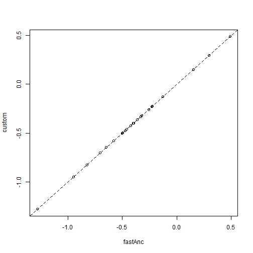
The problem with this method is that it will generally be inefficient at finding the ML solution as the number of nodes in our tree increases, and will even often fail to find the MLE. Luckily for the problem of ancestral state estimation under Brownian motion, relatively simple analytic solutions can be used. Let's take advantage of these to check our custom optimizer. If it worked, they should fall on the 1:1 line:
aa <- fastAnc(tree, x[tree$tip.label])
plot(aa, fit$par[2:length(fit$par)], xlab = "fastAnc", ylab = "custom")
lines(range(x), range(x), lty = "dashed")  ## 1:1 line
One of the most common critiques of ancestral state estimation is that the uncertainty around ancestral states can be large; and, furthermore, that this uncertainty is often ignored. Let's address this by obtaining 95% CIs on ancestral values, and then let's show that the 95% CIs include the generating values around 95% of the time:
## first, let's go back to our previous dataset
fit <- fastAnc(tree, x[tree$tip.label], CI = TRUE)
print(fit)
## $ace
##      27      28      29      30      31      32      33      34      35
## -0.4230 -0.4609 -0.5012 -0.6463 -0.7011 -1.2794 -1.2790 -0.8249 -0.5805
##      36      37      38      39      40      41      42      43      44
## -0.6477 -0.9473 -0.3966  0.1522  0.4888 -0.3974 -0.4942 -0.3624 -0.4739
##      45      46      47      48      49      50      51
## -0.3302 -0.3217 -0.2577 -0.1279  0.2937 -0.2226 -0.2300
##
## $CI95
##       [,1]      [,2]
## 27 -1.2450  0.398894
## 28 -1.0318  0.110035
## 29 -1.0116  0.009128
## 30 -1.1442 -0.148351
## 31 -1.2078 -0.194343
## 32 -1.7537 -0.805028
## 33 -1.7493 -0.808621
## 34 -1.3329 -0.316862
## 35 -0.9933 -0.167790
## 36 -1.2258 -0.069595
## 37 -1.1330 -0.761592
## 38 -0.9381  0.144907
## 39 -0.3542  0.658670
## 40  0.1743  0.803326
## 41 -0.8637  0.068797
## 42 -0.8500 -0.138377
## 43 -0.7901  0.065348
## 44 -0.8291 -0.118600
## 45 -0.8222  0.161744
## 46 -0.7771  0.133587
## 47 -0.7013  0.185842
## 48 -0.4995  0.243718
## 49  0.1486  0.438773
## 50 -0.5231  0.077875
## 51 -0.5253  0.065409
## this is the fraction of time that the true value is within our 95% CI
mean(((x[1:tree$Nnode + length(tree$tip.label)] >= fit$CI95[, 1]) + (x[1:tree$Nnode +
    length(tree$tip.label)] <= fit$CI95[, 2])) == 2)
## [1] 0.84
One small tree doesn't tell us much, so let's repeat for a sample of trees & reconstructions:
## custom function that conducts a simulation, estimates ancestral states, &
## returns the fraction on 95% CI
foo <- function() {
    tree <- pbtree(n = 100)
    x <- fastBM(tree, internal = TRUE)
    fit <- fastAnc(tree, x[tree$tip.label], CI = TRUE)
    mean(((x[1:tree$Nnode + length(tree$tip.label)] >= fit$CI95[, 1]) + (x[1:tree$Nnode +
        length(tree$tip.label)] <= fit$CI95[, 2])) == 2)
}
## conduct 100 simulations
pp <- replicate(100, foo())
mean(pp)
## [1] 0.9483
Cool. Well, this shows us that although CIs can be large, when the model is correct they will include the generating value (1-α)% of the time.
It is also possible to estimate ancestral states using other models of character evolution other than Brownian motion. It is possible to, for instance, estimate ancestral states under the OU model that we have already learned. One note of caution: when the selection parameter (α) is very large, then the ancestral states will all tend towards the same value (the fitted optimum, θ).
For this example, we will use the function anc.ML which permits us to specify an OU model:
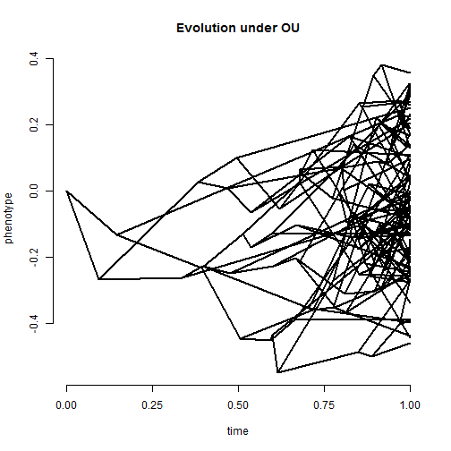
## simulate tree & data under the OU model
alpha <- 2
tree <- pbtree(n = 100, scale = 1)
x <- fastBM(tree, internal = TRUE, model = "OU", alpha = alpha, sig2 = 0.2)
## Warning: alpha but not theta specified in OU model, setting theta to a.
phenogram(tree, x, ftype = "off")
title("Evolution under OU")
## fit the model (this may be slow)
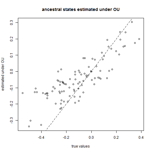
aa <- anc.ML(tree, x[tree$tip.label], model = "OU")
plot(x[1:tree$Nnode + length(tree$tip.label)], aa$ace, xlab = "true values",
    ylab = "estimated under OU")
lines(range(x), range(x), lty = "dashed")
title("ancestral states estimated under OU")
We can theoretically fix the state for any internal node during MLE of ancestral states. In practice, we would do this by attaching a terminal edge of zero length to the internal node we wanted to fix, and then treat it like another tip value in our analyses.
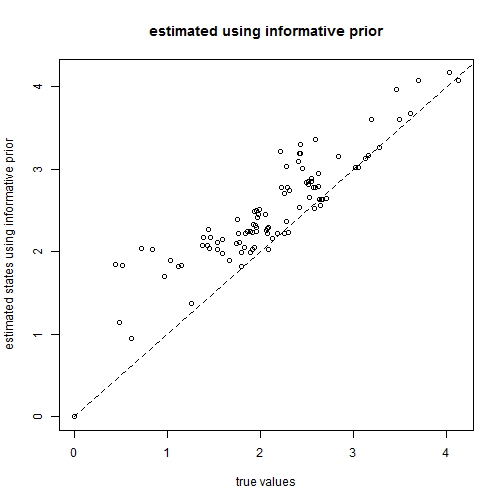
Another possibility, which also allows for the possibility that ancestral states are uncertain, is to use an informative prior probability density on one or multiple states at internal nodes, and then estimate ancestral states using Bayesian MCMC.
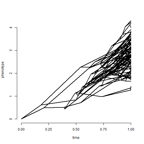
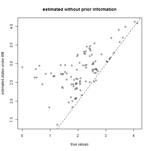
Let's try this using a really bad case for ancestral character estimation from contemporaneous tip data: Brownian evolution with a trend. Note that although we theoretically could do so - we are not fitting a trended model here.
packageVersion("phytools")
## [1] '0.4.10'
tree <- pbtree(n = 100, scale = 1)
## simulate data with a trend
x <- fastBM(tree, internal = TRUE, mu = 3)
phenogram(tree, x, ftype = "off")
## let's see how bad we do if we ignore the trend
plot(x[1:tree$Nnode + length(tree$tip.label)], fastAnc(tree, x[tree$tip.label]),
    xlab = "true values", ylab = "estimated states under BM")
lines(range(x), range(x), lty = "dashed")
title("estimated without prior information")
## incorporate prior knowledge
pm <- setNames(c(1000, rep(0, tree$Nnode)), c("sig2", 1:tree$Nnode + length(tree$tip.label)))
## the root & two randomly chosen nodes
nn <- as.character(c(length(tree$tip.label) + 1, sample(2:tree$Nnode + length(tree$tip.label),
    2)))
pm[nn] <- x[nn]
## prior variance
pv <- setNames(c(1000^2, rep(1000, length(pm) - 1)), names(pm))
pv[as.character(nn)] <- 1e-100
## run MCMC
mcmc <- anc.Bayes(tree, x[tree$tip.label], ngen = 1e+05, control = list(pr.mean = pm,
    pr.var = pv, a = pm[as.character(length(tree$tip.label) + 1)], y = pm[as.character(2:tree$Nnode +
        length(tree$tip.label))]))
## List of 7
##  $ sig2   : num 1.16
##  $ a      : Named num 0
##   ..- attr(*, "names")= chr "101"
##  $ y      : Named num [1:98] 0 0 0 0 0 0 0 0 0 0 ...
##   ..- attr(*, "names")= chr [1:98] "102" "103" "104" "105" ...
##  $ pr.mean: Named num [1:100] 1000 0 0 0 0 0 0 0 0 0 ...
##   ..- attr(*, "names")= chr [1:100] "sig2" "101" "102" "103" ...
##  $ pr.var : Named num [1:100] 1e+06 1e-100 1e+03 1e+03 1e+03 ...
##   ..- attr(*, "names")= chr [1:100] "sig2" "101" "102" "103" ...
##  $ prop   : num [1:100] 0.0116 0.0116 0.0116 0.0116 0.0116 ...
##  $ sample : num 100
aa <- colMeans(mcmc[201:1001, as.character(1:tree$Nnode + length(tree$tip.label))])
plot(x[names(aa)], aa, xlab = "true values", ylab = "estimated states using informative prior")
lines(range(x), range(x), lty = "dashed")
title("estimated using informative prior")
OK. That's it for now.
Written by Liam J. Revell. Last updated May 27, 2014